Project Overview
The objective of this project is to compute and visualize geodesic curves on various surfaces defined by their parametrizations, using Christoffel symbols. For each surface, we carry out the analytical derivation of the geodesic equations as a system of differential equations. We then apply numerical methods to solve these systems and plot the resulting geodesics. Finally, we compare the performance of the methods used and assess which one yields the most reliable results for each surface.
Description of the Mathematical Model
What Is a Geodesic?
A geodesic is the shortest path between two points on a surface or, more generally, in a curved space. In Euclidean geometry, geodesics are straight lines. On curved surfaces, however, they are curves that represent the locally ”straightest” possible paths — generalizations of straight lines in non-Euclidean spaces.
How Do We Find Geodesics?
Given a local parametrization of a surface, we can derive a system of second-order differential equations that describe its geodesics by using Christoffel symbols.
The metric tensor is given by:
Once the Christoffel symbols have been computed, the geodesic equations take the form:
Two equations considered together represent a system of two second order differential equations whose solutions compute geodesics on a surface. So, this system of differential equations is a tool for explicitly obtaining formulas of geodesics on a surface. This system is frequently solved in everyday life, for example when determining the shortest flight route for an airplane.
Derivation of formulas
Geodesics of a Plane
We proceed to derive the geodesic equations for a plane parametrized by
where is a point and are linearly independent vectors. The resulting geodesics should correspond to straight lines on the plane.
Step 1: Inverse of the metric tensor
We first compute the inverse of the metric tensor for the parametrized surface.
The partial derivatives of with respect to the parameters are
The components of the first fundamental form (metric tensor) are given by the dot products of these partial derivatives:
Its inverse is computed by the standard formula for a matrix:
Step 2: Calculation of Christoffel symbols
Next, we compute the Christoffel symbols. Since all second derivatives of the parametrization are zero, it follows that all Christoffel symbols vanish:
Substituting this into the system of differential equations that describe geodesic curves, we obtain:
Integrating both equations once with respect to , we get:
where are constants of integration.
Integrating again, we obtain:
where are additional constants of integration.
Step 3: Parametrization of the geodesic curve on the surface
Finally, we use the results from step two and substitute them into the original parametrization of the surface. Recall that the surface is parametrized by
and from step two we have:
Substituting these into gives:
Distributing terms:
Define:
so that the geodesic curve becomes
This is a straight line in , confirming that geodesics on a parametrized plane are straight lines.
Geodesics of a Sphere
We parametrize a sphere in by the function
where . Note that for a bijective correspondence, the parameters and must lie in the intervals
Step 1: Inverse of the metric tensor
We start by computing the first derivatives of with respect to and , along with their dot products:
Next, we calculate the dot products of these vectors:
Therefore, the first fundamental form (metric tensor) matrix is
and its inverse is
Step 2: Calculation of Christoffel symbols
We begin by computing the second partial derivatives of :
The inverse of the metric tensor from earlier is:
Using the formula for Christoffel symbols of the first kind:
we compute the non-zero symbols (all omitted terms below evaluate to zero due to orthogonality or simplification):
Step 3: Parametrization of the geodesic curve on the surface
Combining the results from the previous step, we arrive at the system of second-order differential equations that describe the geodesics on the sphere:
Substituting the Christoffel symbols, we get:
Step 4: Conversion into a first-order system
The system of differential equations derived in step three is generally difficult to solve analytically. Therefore, we apply numerical methods to find solutions. To use standard numerical solvers, we first convert the second-order system into a system of first-order differential equations.
We define new variables:
This yields the following system of first-order differential equations:
Geodesics of a Torus
Parametrization of the Torus
We parametrize the torus using two angles and , with and . The parametrization is given by:
where is the major radius (distance from the center of the tube to the center of the torus), and is the minor radius (radius of the tube).
Step 1: Inverse of the metric tensor
We first compute the partial derivatives of the parametrization with respect to and :
Now we compute the dot products:
Therefore, the metric tensor is:
Step 2: Calculation of Christoffel symbols
We first compute the second partial derivatives of the parametrization :
The Christoffel symbols (computed as for the sphere) are:
Step 3: Parametrization of the geodesic curve on the surface
Finally, we obtain the following system of second-order differential equations for the geodesic curves on the torus:
We introduce new variables to rewrite the second-order system as a system of four first-order differential equations:
The resulting first-order system is:
Numerical Methods Used
To compute and plot geodesics on the surface, three numerical methods were employed:
- Euler's method,
- Runge-Kutta 4 (RK4) method,
- Dormand-Prince 5 (DOPRI5) method.
Euler's method is a simple, first-order scheme. While it may be effective in special cases, it is generally unstable and introduces significant numerical error, especially when applied to nonlinear systems such as the geodesic equations. A more reliable approach is to use higher-order or adaptive methods.
Runge-Kutta 4 is a fixed-step, fourth-order method, offering a good balance between accuracy and computational cost. Dormand-Prince 5, on the other hand, is a fifth-order adaptive method. It dynamically adjusts the step size based on local error estimates, improving efficiency and stability in regions where the solution changes rapidly.
In general, the global truncation error of a numerical method of order behaves like , where is the step size. This means that halving the step size reduces the error by a factor of approximately . For example:
- Euler's method (order 1): error scales as ,
- RK4 (order 4): error scales as ,
- DOPRI5 (order 5): error scales as .
Thus, both RK4 and DOPRI5 are expected to outperform Euler's method in terms of accuracy for most cases, particularly when the geodesic path exhibits rapid curvature or complex behavior.
Source Code Description
What follows are explanations of critical source code functionalities contained in the supporting Julia source code file, that were used to put all the theoretical concepts from the previous section into practice.
Euler’s Method
The function euler(f, Y0, tspan, h, p) accepts five arguments: a function representing the geodesic equation for the surface, the initial condition vector , the time interval tspan, the step size , and the parameter tuple .
The initial condition has the form:
where and specify the starting point on the surface in parameter coordinates, and the corresponding derivatives specify the initial direction of the geodesic.
The function's output are the array of steps taken and the array of values of the geodesic at each step.
function euler(f, Y0, tspan, h, p)
    t0, tk = tspan
    t = t0:h:tk
    Y = [Y0]
    du = similar(Y0)
    for ti in t[1:end-1]
        f(du, Y[end], p, ti)
        push!(Y, Y[end] + h * du)
    end
    return t, Y
end
Runge-Kutta 4
The function accepts parameters in the same manner as Euler's method described in subsection Euler’s Method. Its output format is also identical, returning the time steps and the geodesic values at each step. However, it is immediately clear that more computations are involved in each iteration, reflecting the increased accuracy of the fourth-order method.
function rk4(f, Y0, tspan, h, p)
    t0, tk = tspan
    t = t0:h:tk
    Y = [Y0]
    du = similar(Y0)
    for ti in t[1:(end-1)]
        f(du, Y[end], p, ti); k1 = h * du
        f(du, Y[end] + k1/2, p, ti + h/2); k2 = h * du
        f(du, Y[end] + k2/2, p, ti + h/2); k3 = h * du
        f(du, Y[end] + k3, p, ti + h); k4 = h * du
        push!(Y, Y[end] + (k1 + 2*k2 + 2*k3 + k4)/6)
    end
    return t, Y
end
Dormand-Prince 5 (DOPRI5)
The Dormand-Prince 5 method is imported from the Julia package DifferentialEquations.jl. The numerical solution procedure consists of first defining the problem using the ODEProblem constructor, followed by solving it with the solve function. The results are stored in a solution object, from which both the time steps and corresponding geodesic values can be extracted for plotting.
A stringent tolerance of is used for both absolute and relative errors to ensure high precision. Tolerances looser than approximately can lead to noticeably imprecise geodesics.
To make the solution comparable with fixed-step methods, the option saveat=t_eval is specified, restricting the saved output to fixed time points defined by the vector t_eval. This allows consistent sampling of the solution for visualization and further analysis.
using DifferentialEquations

# Define the ODE problem
prob = ODEProblem(geodesic_torus!, Y0, tspan, p)
# Set evaluation points for solution saving
t_eval = 0:0.01:3.5
# Solve using Dormand-Prince 5 method with strict tolerances
sol = solve(prob, DP5(), abstol=1e-12, reltol=1e-12, saveat=t_eval)
# Extract time steps and geodesic values
t = sol.t
Y_matrix = hcat(sol.u...)'
Results
Sphere
Initial Conditions
We test three different initial conditions representing geodesics on the sphere:
- Equatorial geodesic:
- Meridional geodesic:
- Diagonal geodesic:
For each initial condition, three step sizes were used: , , and .
Equatorial Geodesic
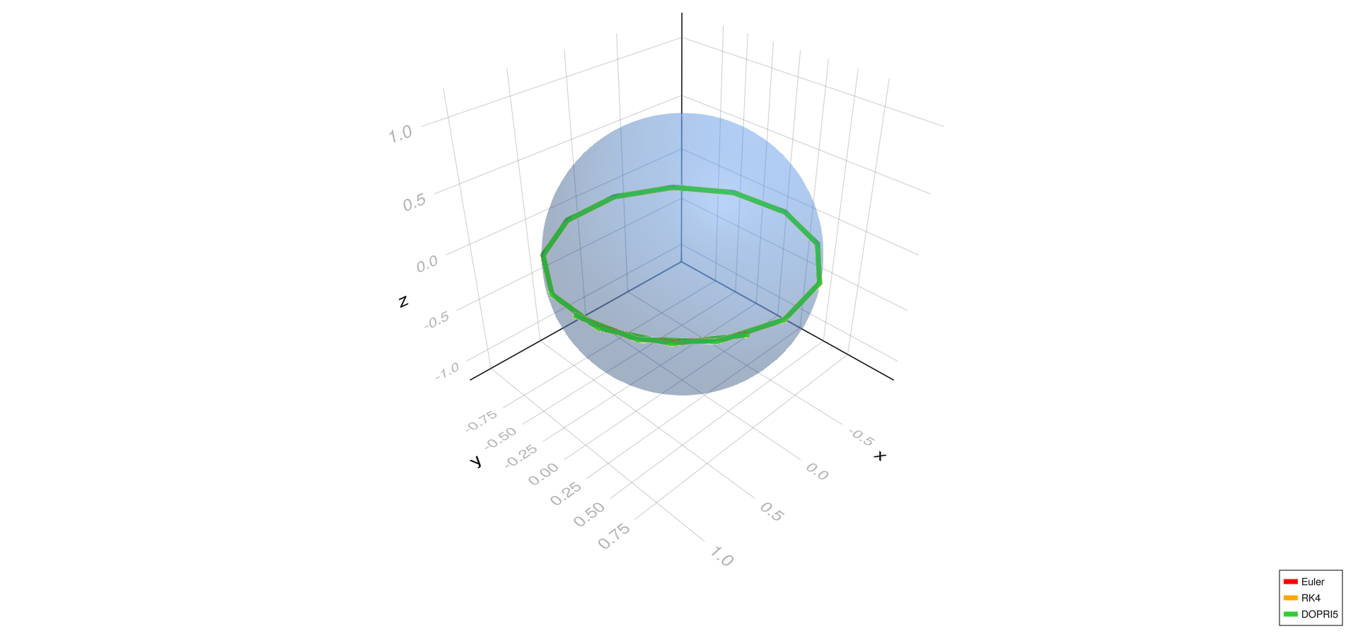
Equatorial geodesic,
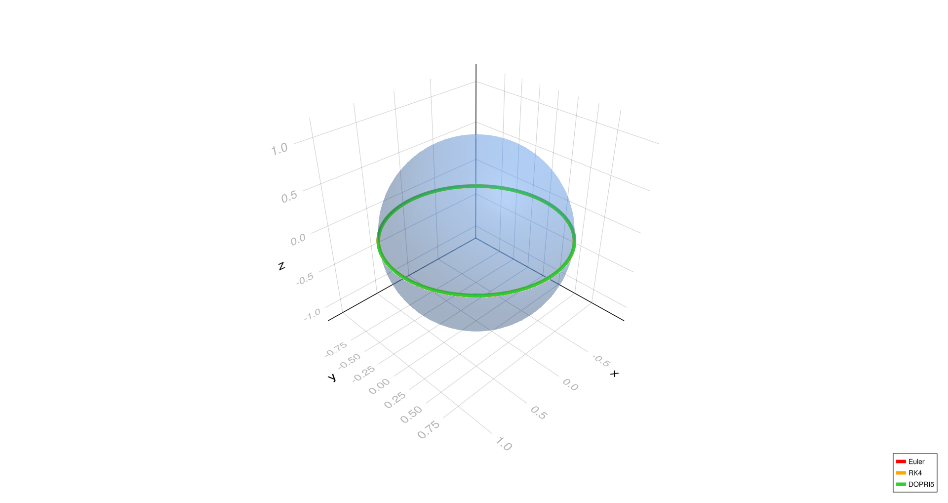
Equatorial geodesic,
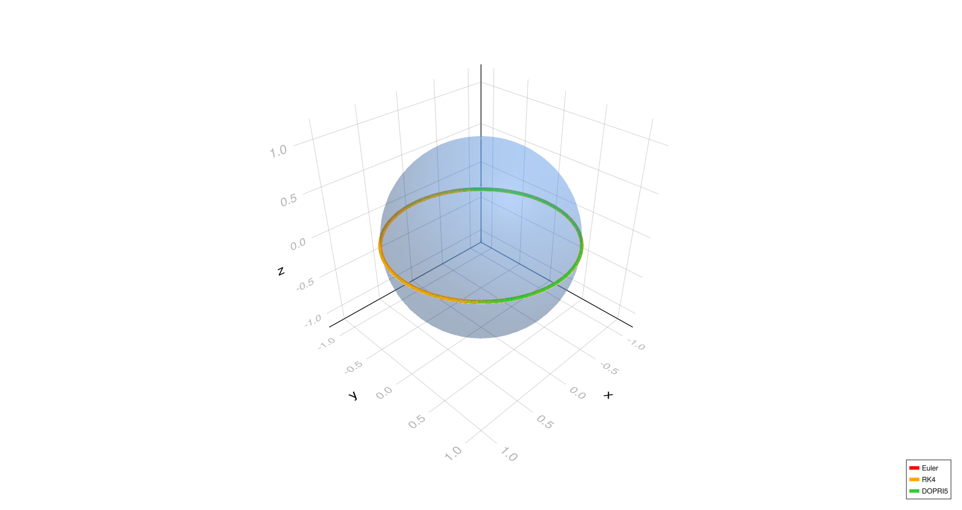
Equatorial geodesic,
Meridional Geodesic
Meridional geodesic,

Meridional geodesic,
Meridional geodesic,
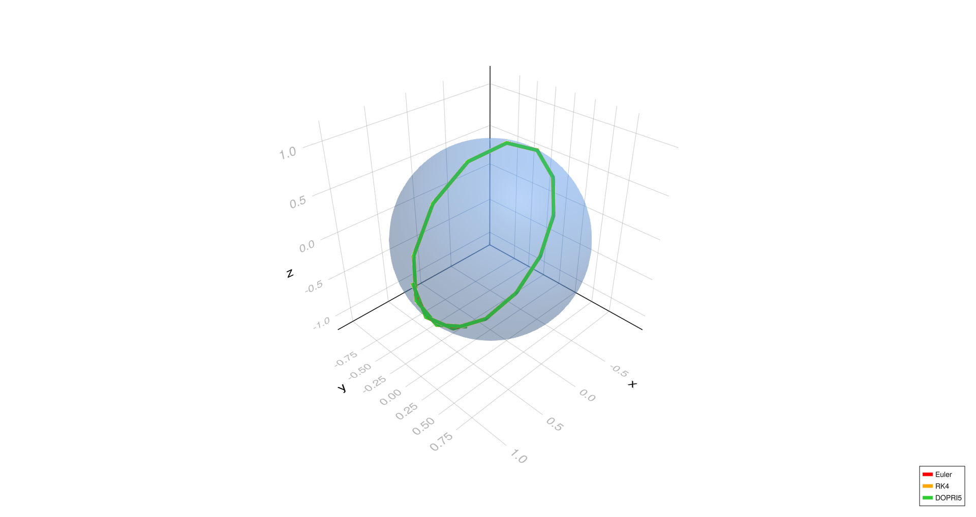
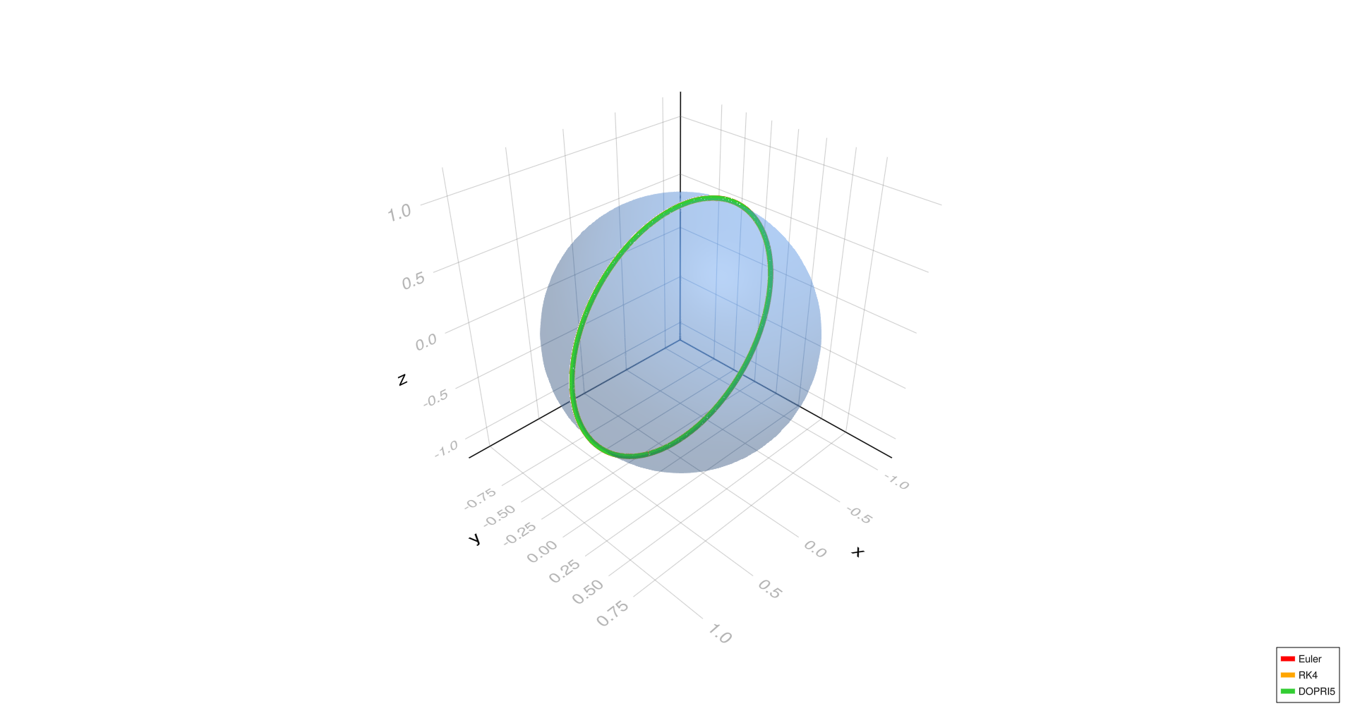
Diagonal Geodesic
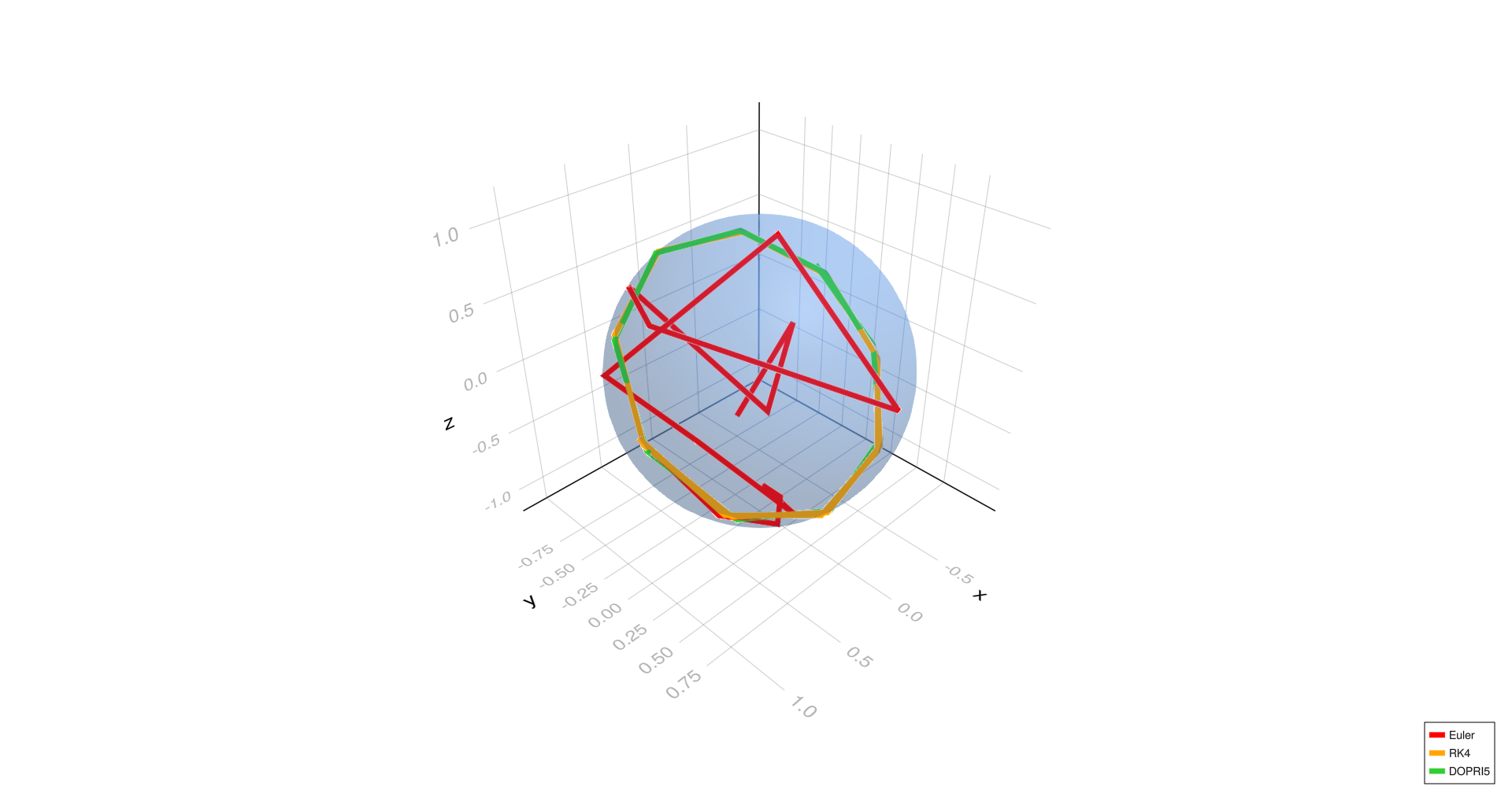
Diagonal geodesic,
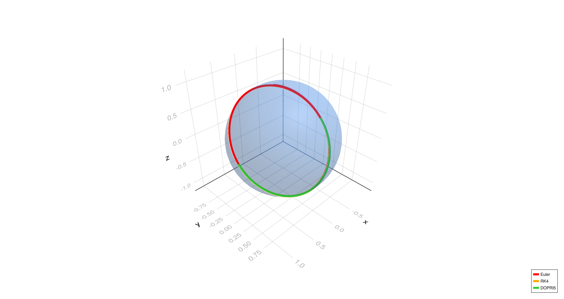
Diagonal geodesic,
Diagonal geodesic,
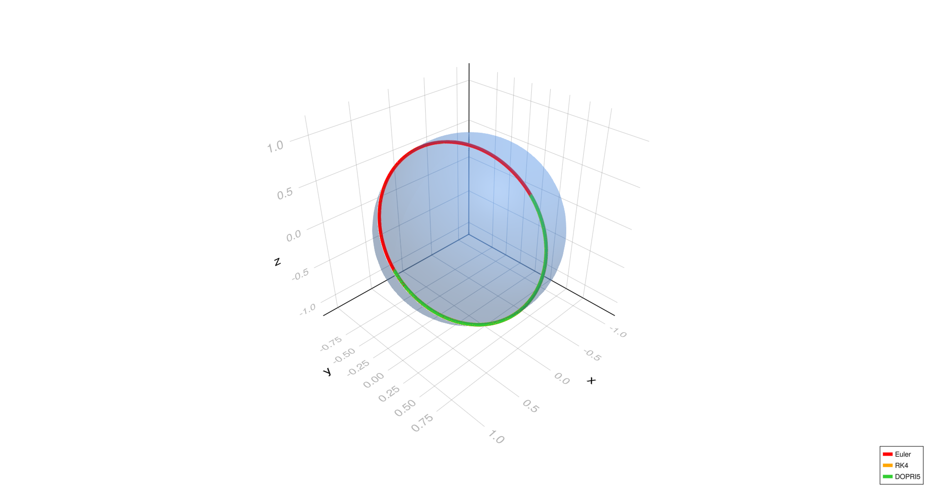
Diagonal Geodesic (Detailed Views)
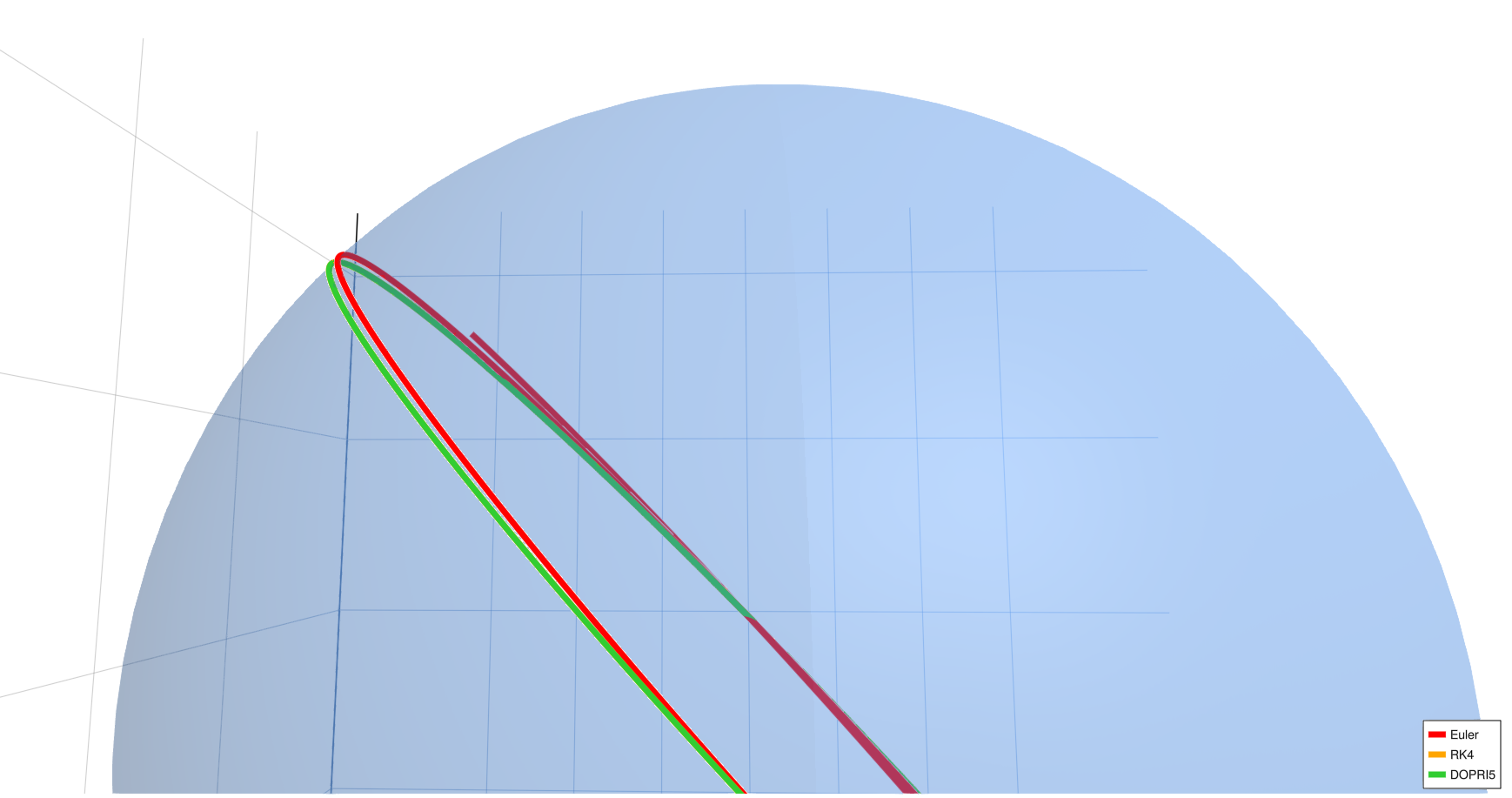
Diagonal geodesic, (detailed view)
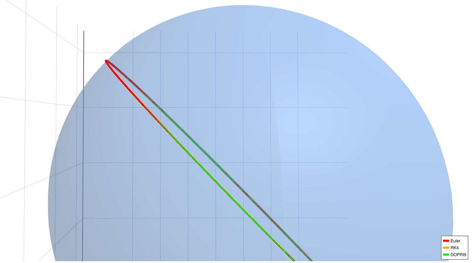
Diagonal geodesic, (detailed view)
Empirical Observations
- The equatorial and meridional geodesic cases show excellent agreement among all three methods (Euler, RK4, DOPRI5) at all step sizes, indicating stable geodesics.
- For the diagonal geodesic case, Euler's method deviates noticeably at (h = 1.0) and slightly at (h = 0.01), while RK4 and DOPRI5 remain well aligned.
- At the finest step size (h = 0.0001), all methods align closely even in the diagonal case, confirming that reducing step size improves Euler's accuracy.
Torus
Initial Conditions
We test six distinct initial conditions representing geodesics on the torus:
- Inner equator:
- Outer equator:
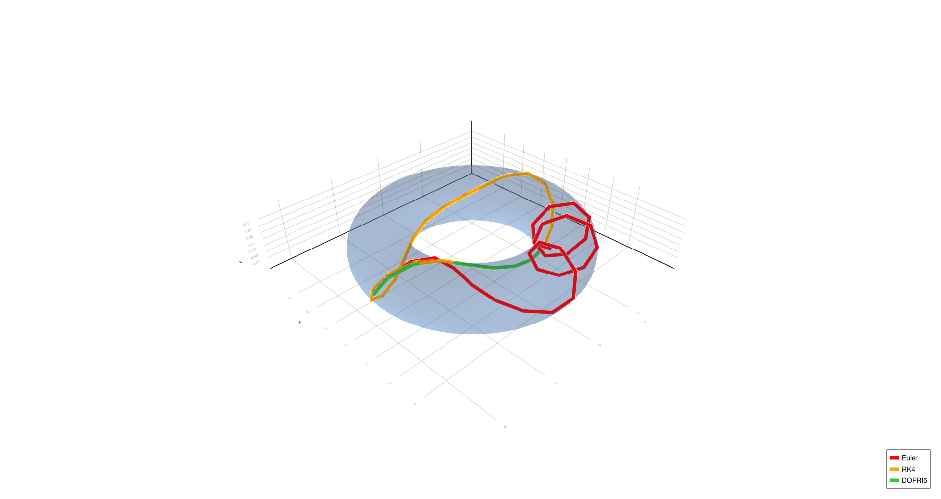
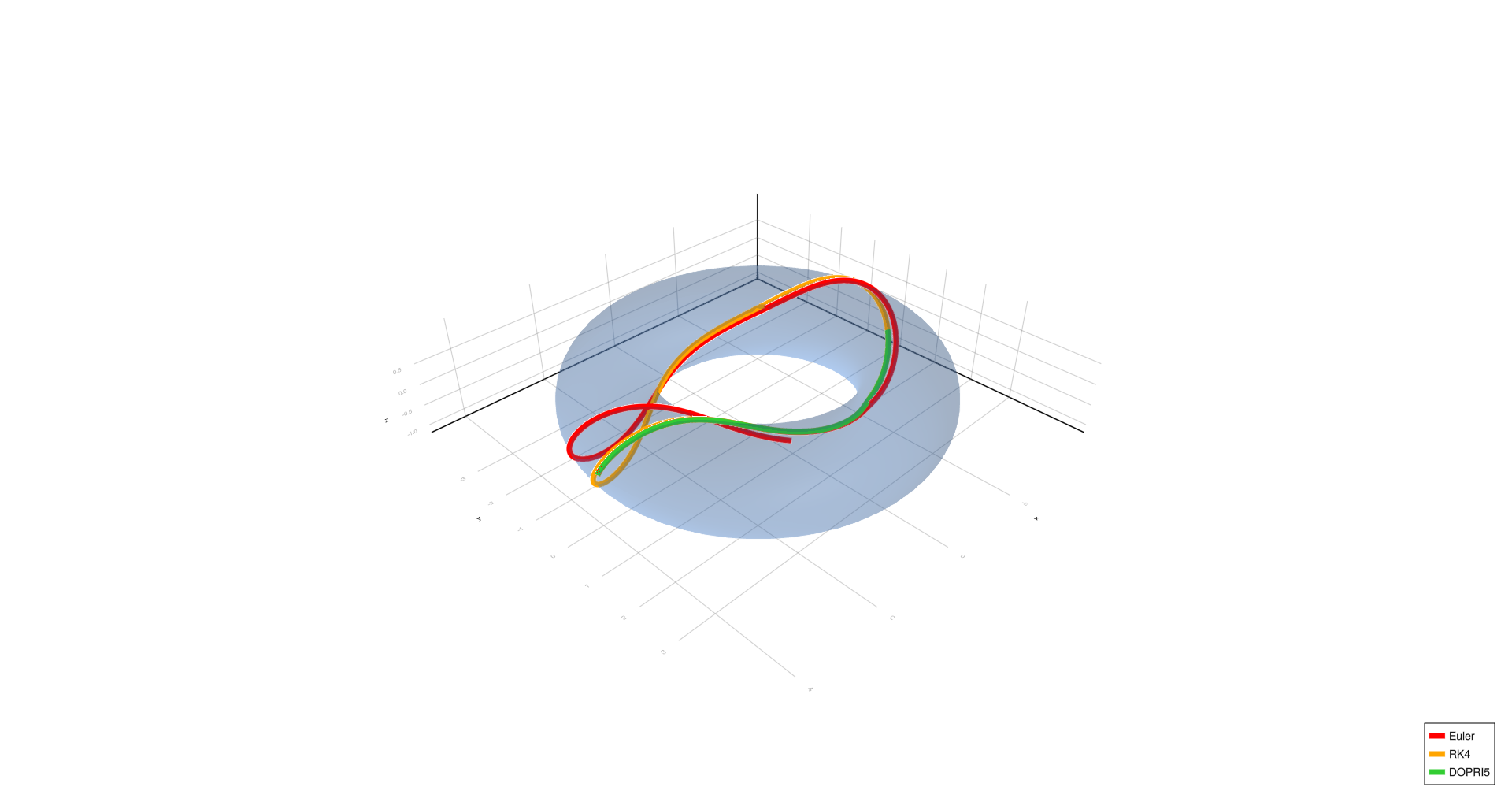
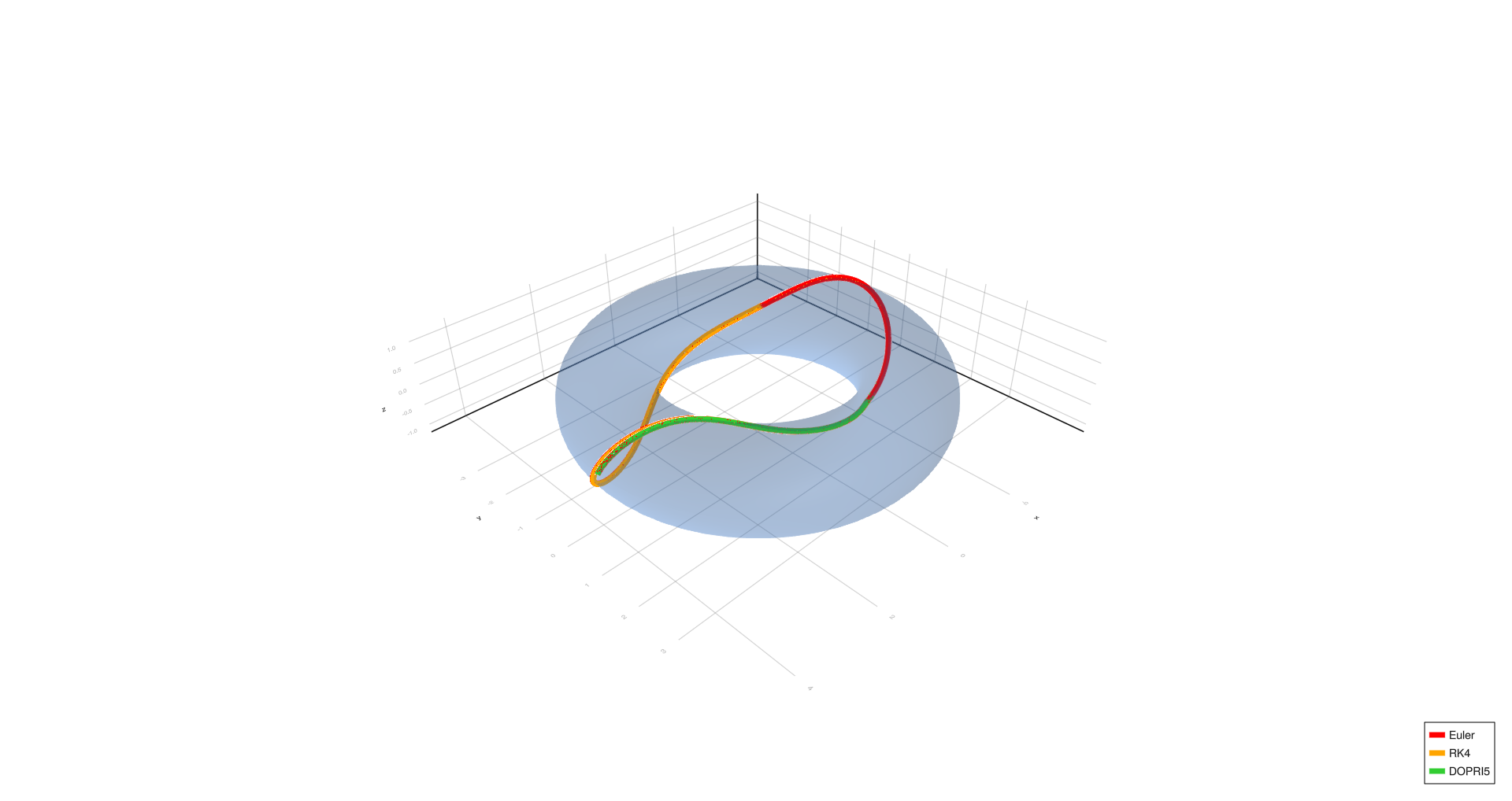
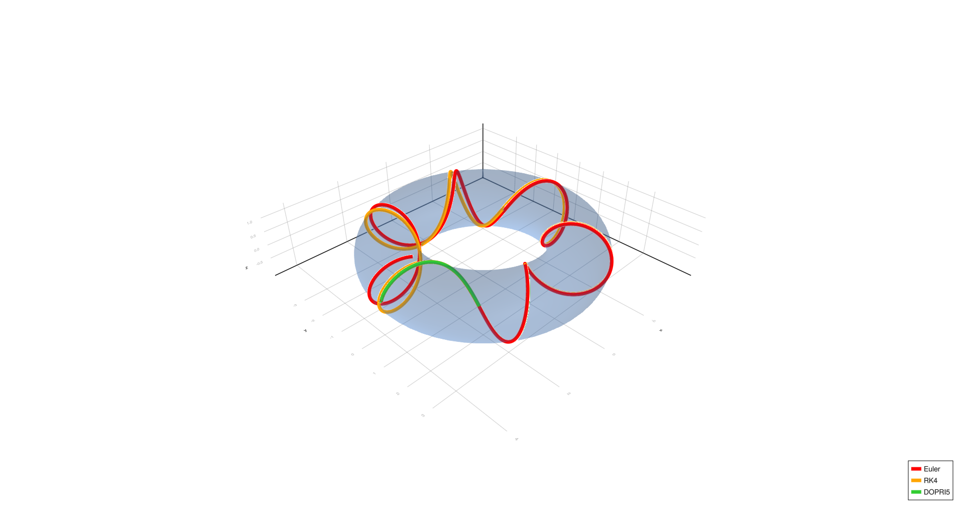
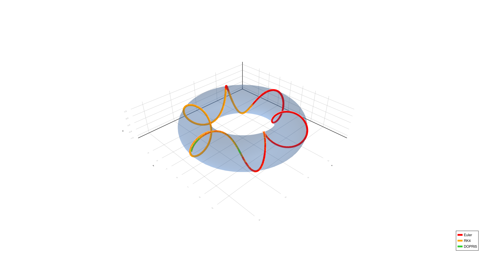
- Four turns:
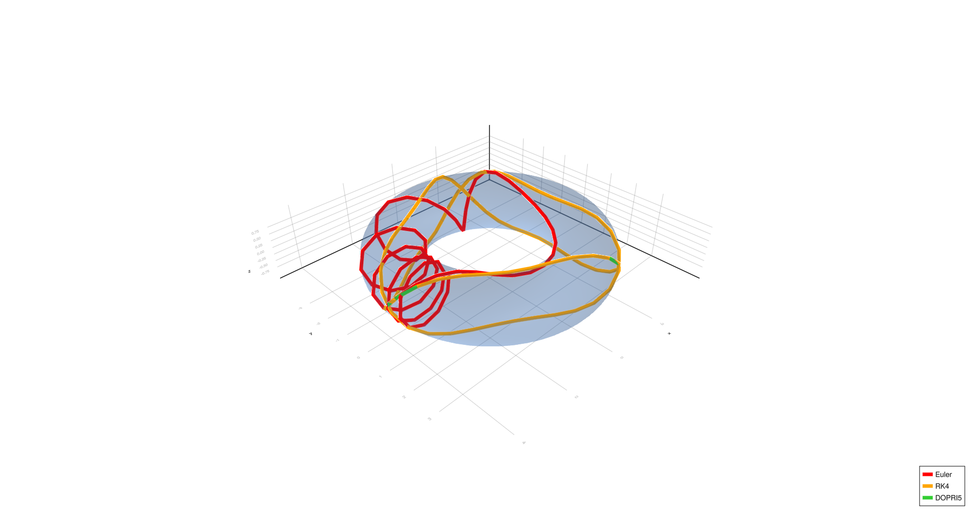
- Complex spiral:
- Six turns:
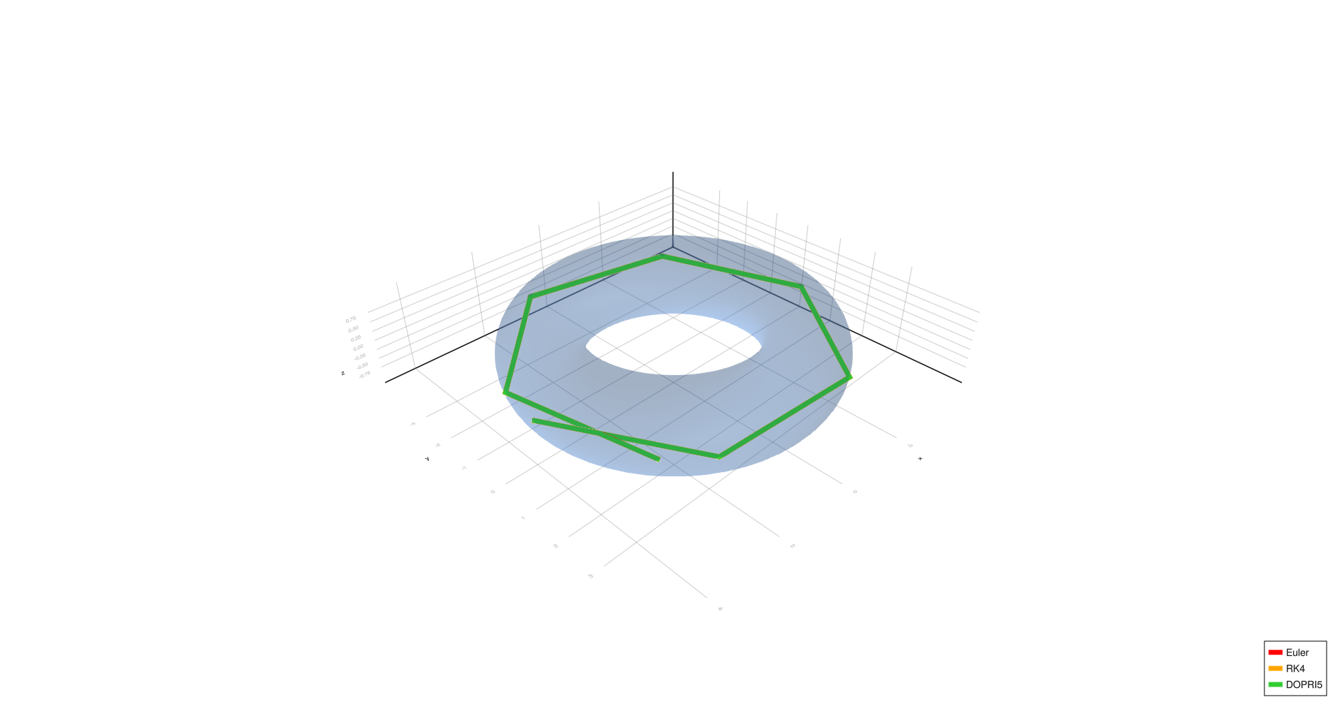
- Triangle:

Inner equator,

Inner equator,
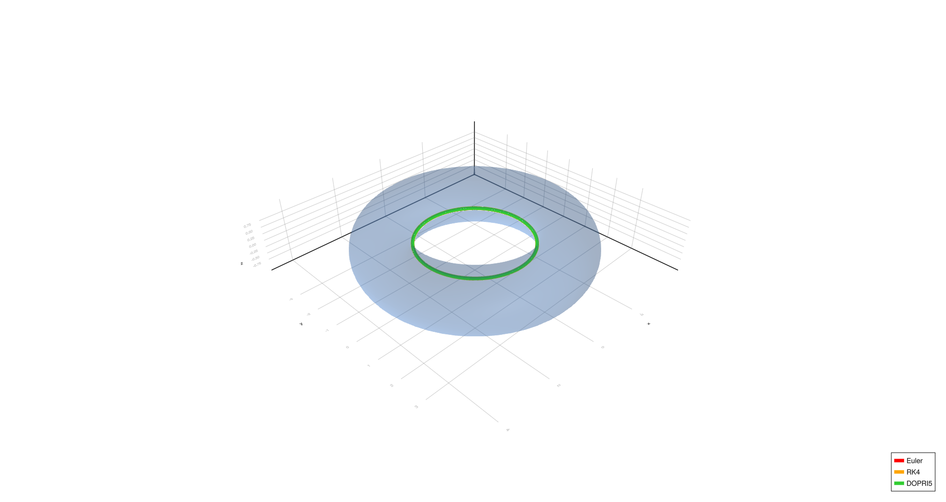
Inner equator,
Outer equator,
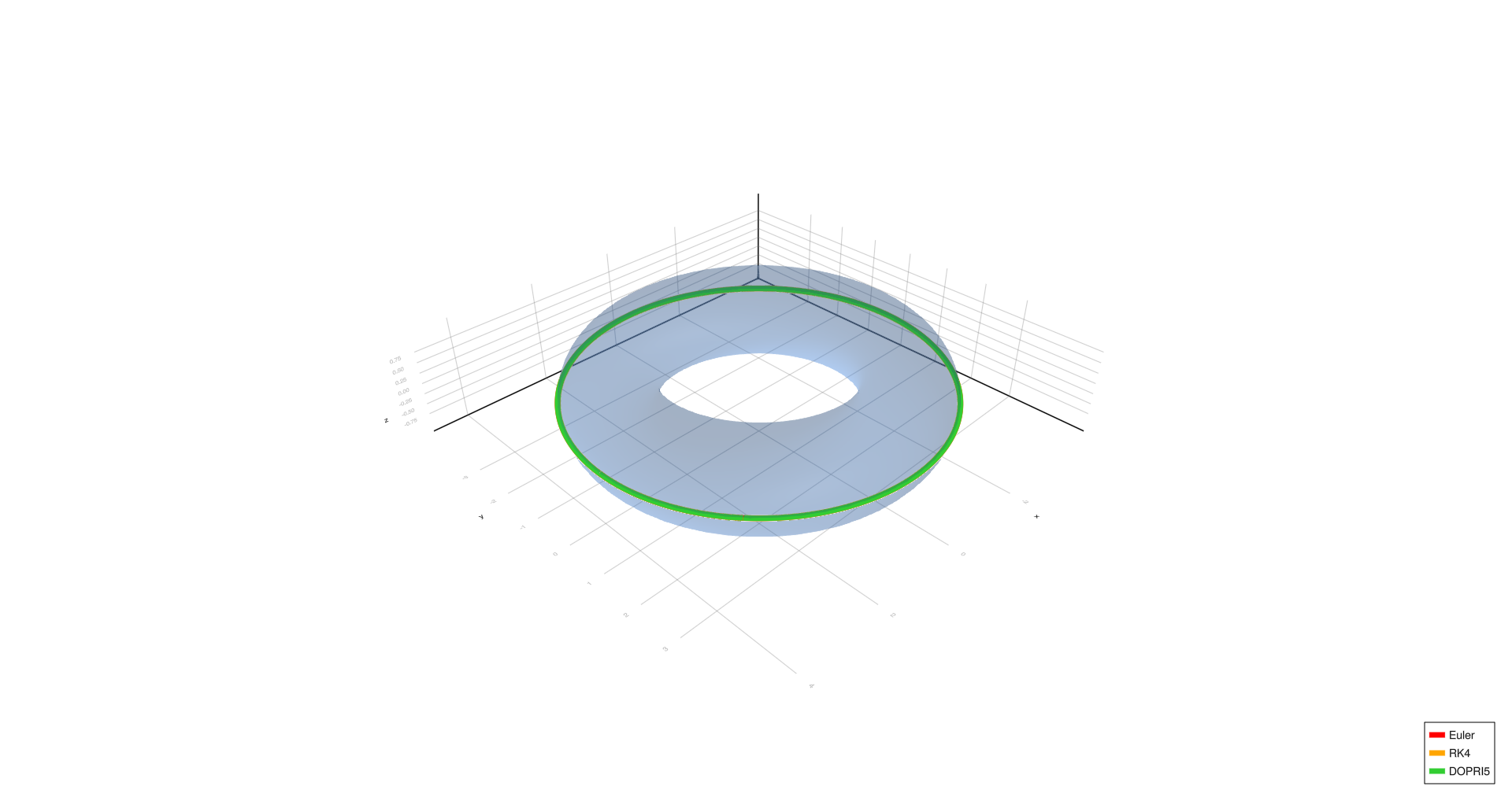
Outer equator,

Outer equator,
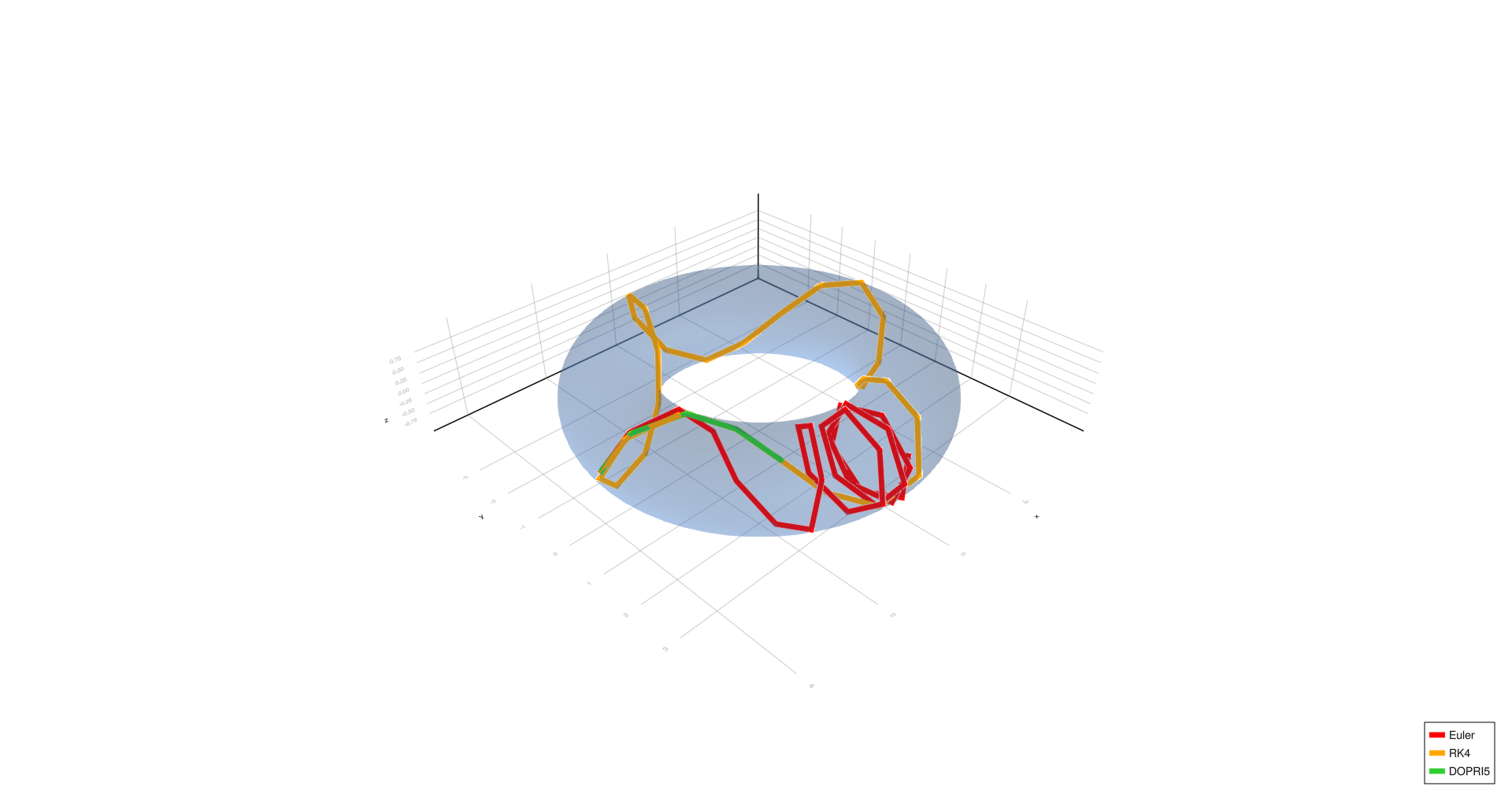
Four turns,
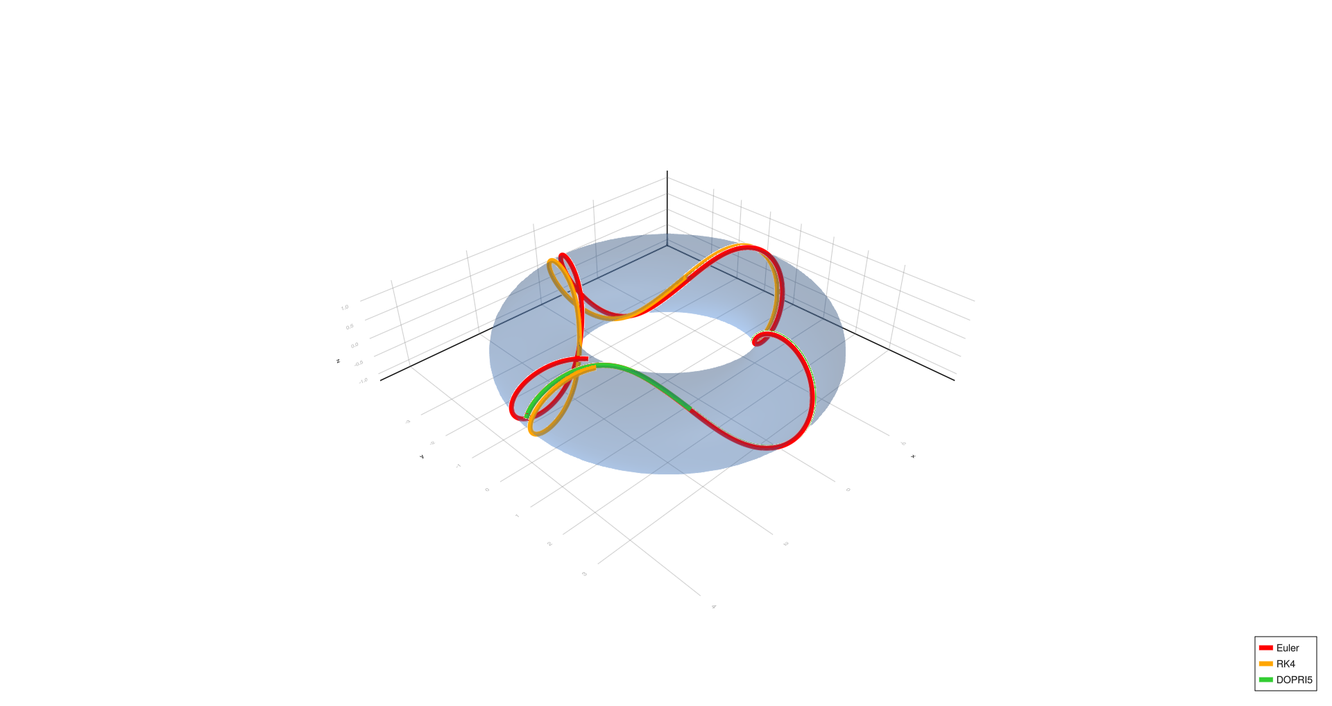
Four turns,
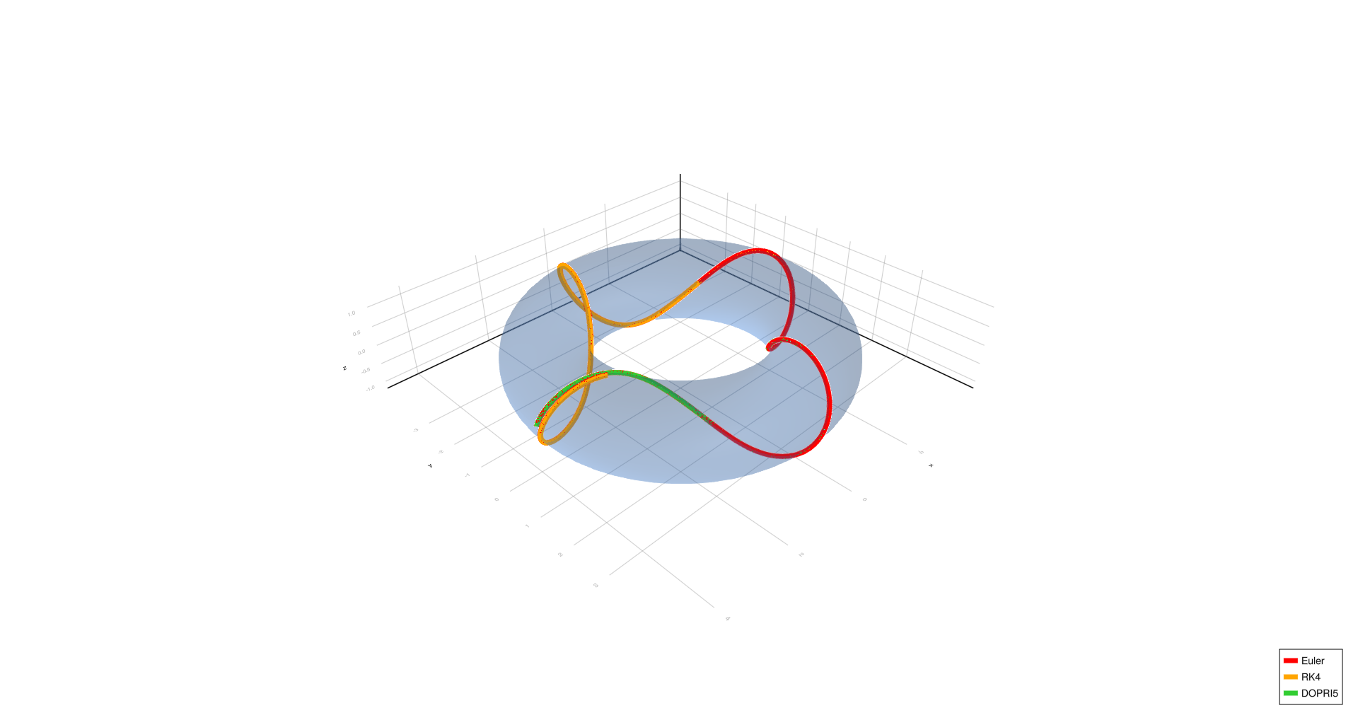
Four turns,
Complex spiral,
Complex spiral,
Complex spiral,
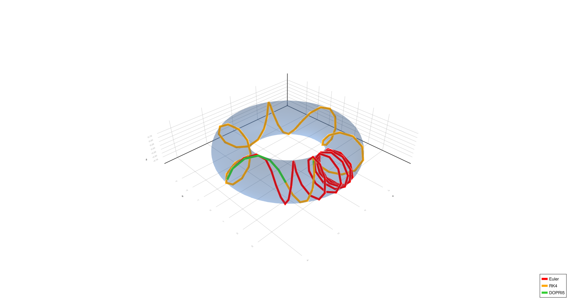
Six turns,
Six turns,
Six turns,
Triangle,
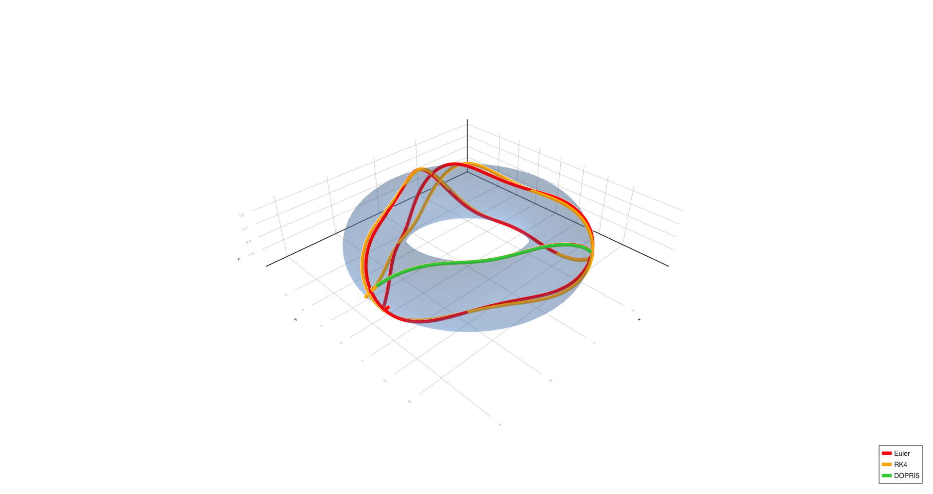
Triangle,
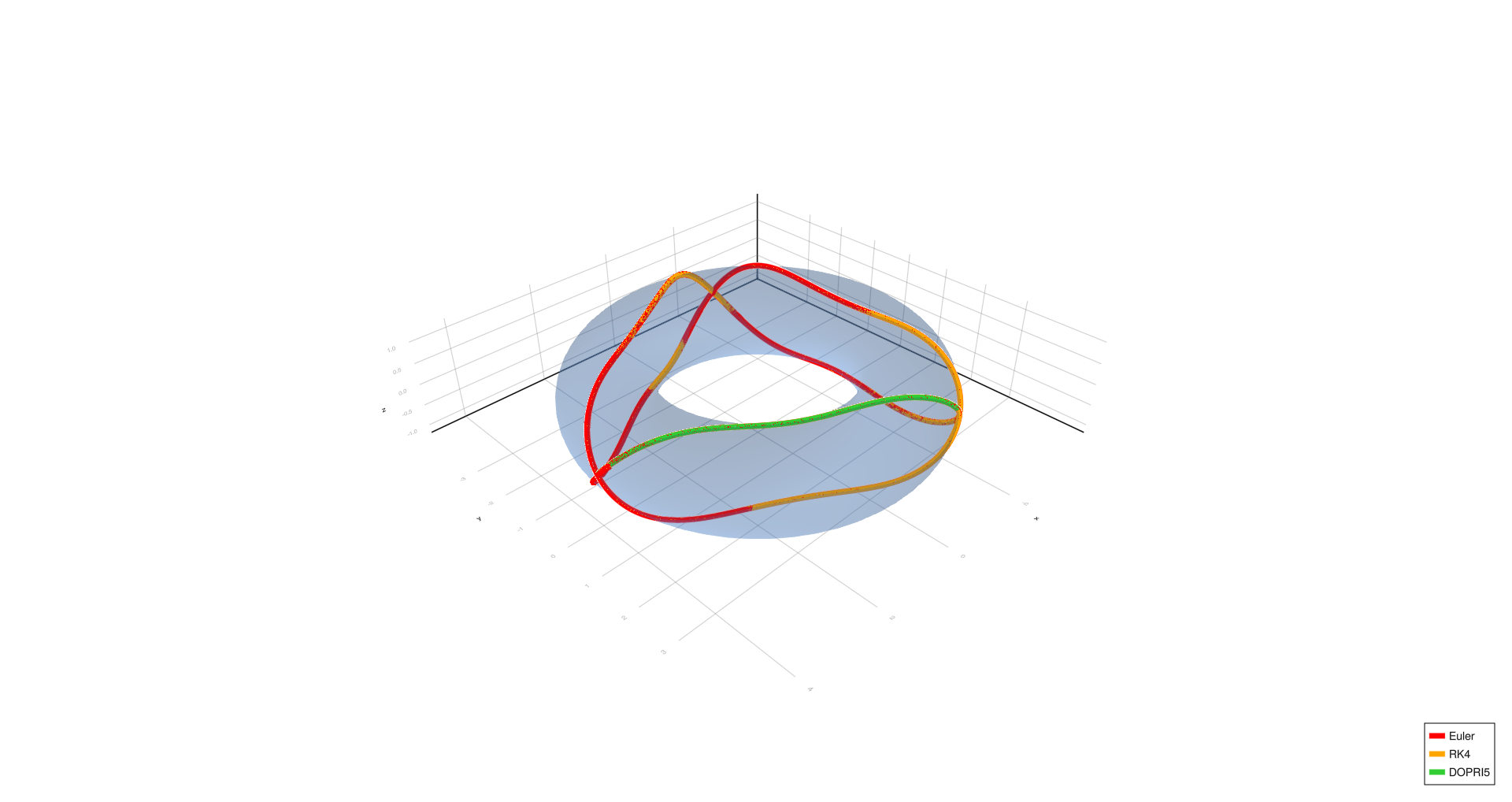
Triangle,
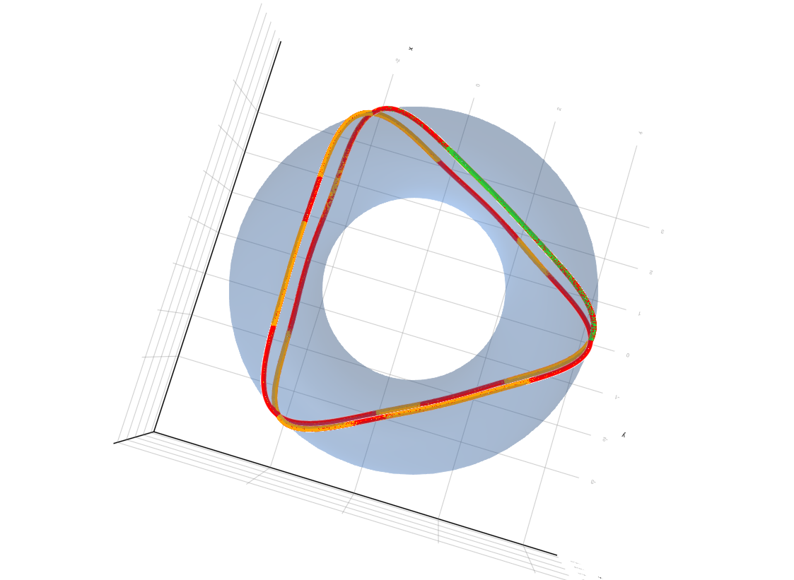
Triangle, (from above)
Empirical Observations
- Inner and outer equators remain stable across all step sizes and methods.
- Four turns, complex spiral, six turns, and triangle show significant deviation with Euler at (h = 1.0), partial correction at (h = 0.01), and convergence with RK4/DOPRI5 at (h = 0.0001).
Conclusion
To compute geodesics accurately, higher-order methods such as Runge-Kutta 4 (RK4) and Dormand-Prince 5 (DOPRI5) are the most reliable. In our experiments, their results were nearly identical, with no practical difference in performance.
While simpler methods like Euler's method can match the precision of higher-order methods in specific, uncomplicated cases, they are generally outperformed. However, reducing the step size significantly (e.g., to (h = 0.0001)) allows even Euler’s method to approach the accuracy of RK4 and DOPRI5.
This presents a clear trade-off: Euler’s method is easy to implement but requires very small step sizes to achieve high accuracy, resulting in increased computational cost. Conversely, RK4 and DOPRI5 are more complex but provide stable and accurate results even with larger step sizes (e.g., (h = 0.01)), making them more efficient overall for most applications.
References
-
Kovač, Gregor. (2023). Sledenje žarku v neevklidskih prostorih. [Diplomsko delo, UL FRI]. Retrieved from https://repozitorij.uni-lj.si/Dokument.php?id=172611&lang=slv
-
Dawkins, Paul. (2022). Section 2.9: Euler's Method [Article, Lamar University]. Retrieved from https://tutorial.math.lamar.edu/classes/de/eulersmethod.aspx
-
eigenchris. (2018). Tensor Calculus 15: Geodesics and Christoffel Symbols (extrinsic geometry) [Video]. Retrieved from https://www.youtube.com/watch?v=1CuTNveXJRc
-
Irons, Mark Lawrence. (2005). The Geodesics of the Torus [Article]. Retrieved from http://www.rdrop.com/~half/math/torus/geodesics.xhtml
-
Vas, Lia. (n.d.). Differential Geometry Handouts. [PDF files, Dept. of Mathematics, Saint Joseph's University]. Retrieved from https://liavas.net/courses/math430/